|
 |
| |
SeaSondes See Japan Tsunami
on
Two Continents
|
 |
Attend the
Tsunami
Detection
Presentation
by Dr. Barrick
at
Oceans ’11 Kona |
SeaSonde HF radars have been providing real-time
data to agencies in several countries on both sides of
the Pacific Ocean for more than a decade. This wide
distribution made them well placed for detecting the March 2011
tsunami in a variety of locations and configurations. This article highlights
several methods, radar frequency bands, and tide gage sensor measurements
that all confirm the validity and robustness of SeaSonde tsunami detections.
Tsunami Detected by Multiple HF Bands
Two High-Res (42 MHz) SeaSondes installed on Hokkaido, northernmost of
Japan’s four main islands, were the closest to the earthquake epicenter and
the first HF radar systems to observe the tsunami - as shown in the figure on
the cover. Being close to the source, the ~40-minute period was clearly visible
in the SeaSonde-observed surface current velocity data from both sites. Nine
hours later and over 8000 km away, Mid-Range (13 MHz) and Long-Range (5
MHz) SeaSondes on the West Coast of the Continental U.S. were also
observing the tsunami signature.
|
|
|
More complexity was observed in the measured periods (25 - 40 min) in
the U.S. due to multiple paths and directions of arrival - as illustrated by
the NOAA http://nctr.pmel.noaa.gov/ tsunami wave energy map (shown
at right). In all cases, the tsunami was observed at three different stages
of current velocity processing and by sensors independent from the
SeaSondes, as described below.
Tsunami Signatures Confirmed by Coastal Tide Gages
How do we know for certain we saw the tsunami? Tide gages on the coast
give water level and, in the U.S., data from these are made available to the
public by NOAA via website. Tide gages are meant to respond to the
slowly varying tides with diurnal and semi-diurnal periods, but they see
the tsunami signals very well. What do the tide gages tell us?
• Both sensors show a slowly varying tidal background until the tsunami
arrived, when both observed the more rapid 25-40 minute period
response - as shown below.
• Signals at the coast on the tide gages were delayed from those recorded
by the radar offshore, from 10 to 30 minutes. The tide gages verified the
SeaSondes were, in fact, capturing the tsunami event. One may ask the
question why do SeaSondes measure the tsunami before the nearby tide
gages do?
• The signals in the current seen by the radars offshore were further “upstream” toward the tsunami source. As it traveled across
the ever-shallower water to get to the coast, it slowed down, as predicted by wave theory, over the path distances from 25 - 40 km.
|

|
• A quarter-cycle delay happens near shore between velocity and height. If the water starts at normal height and velocity begins to
push the mass of water toward shore, it takes time for the height to increase. When the tsunami height reaches its maximum
level, velocity must be zero or the height would continue to increase. For ~40 min period, the quarter cycle delay is ~10 minutes.
• The delay seen by the West coast radars and tide gages is about nine and a half hours, which is exactly as predicted for travel
time across the Pacific based on both models and observations.
|
 |
 |
| Radial current velocity measured from
SeaSonde at Commonweal, 25 km Northwest
of Golden Gate Bridge in California |
Water level observed in San Francisco under
Golden Gate Bridge |
|
Optimum Sampling and Conditions for Tsunami Detection
There is a tradeoff between how often a radar can output information (temporal sampling resolution) and the increment of the
observable data (velocity resolution). Since a tsunami is a hazardous event, it is natural to want the highest sampling rate
possible. Theory and experience has proven, however, that if the velocity sampling is too coarse, it is of little or no value. For
any 13 MHz radar regardless of its make or brand, a 30-second output means the best possible velocity resolution is 38 cm/s.
This is nearly useless, because the tsunami generated currents seen by all of the radars had crest/trough values more like 10-20
cm/s. Using 4 minute outputs gives about 3.5 cm/s resolution, which does a nice job. With this sampling rate, 10 samples were
available per tsunami period, which is more than adequate. The CODAR tsunami detection approach does not force any fixed
sampling rate. Instead, several output rates (velocity resolutions) are computed simultaneously to maximize the possibility of
detection and it has zero impact on standard current processing operations.
In addition to sampling rate, observation time before the tsunami reaches shore depends on water depth -- the shallower and
longer the shelf, the greater the time to reach shore. Unlike the Mid-Atlantic states along the Eastern seaboard, both Japan
and the U.S. West coast are not optimal with narrow shelves of shallow water. Yet, the tsunami was seen in all cases at
distances to 20 km and water depths to 200 m. |

|
• 2-D Current Maps: The HF radar output with which everyone is familiar are current vector
maps requiring two or more coastal radars combining data. 2-D velocity fields show the onset of
tsunami-generated currents is in figure at left. This method has the advantage of producing a
nice image of the currents that is easily interpreted visually, but requires data to be transmitted
between two or more sites and extra processing time. It is most useful for post-processing and
analysis, but not real-time tsunami detection.
• Radial Velocity Maps Radial velocity currents from a single site provide robust data for
tsunami detection and are the basis of CODAR SeaSonde Tsunami Software. Certainly the
individual vectors can be post-processed to observe tsunami effects. More useful to quickly
detect the onset of a tsunami is the CODAR tsunami detection pattern recognition software,
which resolves the radial velocities sensed by a single radar into strips parallel to the bathymetry
contours. Physics forces the velocity vectors to be essentially perpendicular to these contours,
regardless of the direction of the epicenter source. Indeed, velocities resolved in this manner
show the tsunami period, and also the variation with distance offshore that is expected.
• Doppler Sea Echo Stepping back even further in the processing stream (before the direction finding
method is applied and radial velocity maps are made), we looked at the variation in the
width and centroid of the Doppler sea echo with time as a direct measure of the overall tsunami
current. The results of this are illustrated in the time series figures shown above. This stage of
processing is even faster to reach than radial maps and is the focus of future improvements to
CODAR SeaSonde tsunami detection.
HF Radar Tsunami Detection First Described by CODAR
It was over 32 years ago that Barrick first described how an approaching tsunami could be
measured from its HF radar-observed current pattern in a 1979 Remote Sensing of
Environment article. With few HF radars operating at that time and sizable tsunamis being a
rare or infrequent occurrence, this research went largely unnoticed for many
years. Following the 2004 Indian Ocean tsunami, Lipa and Barrick revisited the topic by
developing a tsunami pattern recognition algorithm that worked against the ambient
background flows. The methods described in their 2006 paper formed the basis for the first
and only commercial HF radar tsunami detection software
package available on the market.
|

| On The Radar: South Korea |
Those who regularly read our newsletter know that we like to devote some
space to showcasing the unique activities or research interests of
SeaSonde users. This time, it occurred to us to showcase the activities of
not just one particular customer, but those of an entire country. South Korea is
nearly urrounded by water with the Yellow Sea (West Sea) to the West, the Sea
of Japan (East Sea) to the East and the East China Sea and Korea Strait to the
South. These bodies of water are shared with North Korea, China, Japan and
Russia with the economies of each heavily reliant on them for shipping,
aquaculture and tourism, among others. It makes sense, then, that South Korea
has emerged as one of the most active countries in the world in building a
national surface current monitoring program. By the end of 2011, South Korea
will have more SeaSondes than any country outside of the U.S. and will lead
the world in HF radars per length of coastline. South Korea’s introduction to
HF radar current mapping came in 1992 when some of the first SeaSonde
production units were used in a short term demonstration near Kunsan for the Korean Ocean Research and Development Institute
(KORDI). Several years later, the first units were purchased by Dr. Jae-Chul Lee of Pukyoung University in Busan. Since then, SeaSondes
have been providing real-time current maps and wave parameters for a variety of customers and purposes all around this country.
SeaSonde Networks in Korea Today
Dr. Sang Ho Lee of Kunsan National University owns and operates a SeaSonde network
that is mapping surface currents outside of the Saemangeum Sea Wall, the longest seawall
in the world, located on South Korea’s west coast. The sea wall was built between the
Yellow Sea and the Saemangeum estuary as one of the largest land reclamation projects in
history at 410 km2. Dr. Lee’s research has shed light on the effect the new seawall has on
the circulation outside of the estuary. Since 2007, Dr. Kyung Tae Jung of KORDI and his
team have studied the structure of changed flow after Saemanguem Sea Wall construction
with Kunsan National University. Moreover, they introduced another SeaSonde network
and finished studies to observe the current structure inside the
Straits of Jeju.
The Korea Hydrographic and Oceanographic Administration (KHOA) is engaged in more
operational pursuits, providing real-time data to a wide variety of end-users. Since KHOA
installed SeaSondes near Incheon for the first time in 2002, they have continued to add
new SeaSonde sites. Presently, KHOA owns and operates 4 SeaSonde sites in Yeosu Bay
and 2 sites in Busan New Port. Yeosu Port is one of the major harbors having heavy traffic
and Busan New Port, recently opening big container terminals, is emerging as a main logistics hub port.
This year KHOA plans to install four additional SeaSonde sites for the purpose of monitoring Tsushima current running between Busan
and Tsushima Island. In 2012, they plan to establish and manage a portal hub linking to the HF radar sites of several universities and
institutes, expecting an efficient and united national radar data product display service.
National Dialogue
While today’s HF radar community in South Korea is spread across university and government entities
engaged in both academic and operational pursuits, the diverse community members still effectively
manage to exchange information and share experiences. Currently, Ocean Radar Forum, composed of 20
people, holds a workshop for experts every year to discuss each institution’s plan and newly developed
technology. Oceantech -- the long-standing local sales and service partner of CODAR -- is sharing
information through this kind of regular meeting and providing technical support for many research
institutes and universities allowing efficient SeaSonde operation. Furthermore, Oceantech plans to
assume the O&M responsibility for 10 SeaSonde stations from KHOA later in 2011.
International Collaboration
The South Korea HF radar community has not only been focused on their own research
interests and development but have also been forming collaborative partnerships globally. This
has most recently resulted in a Korean delegation participating in the April 2011 Radiowave
Operators Working Group (ROWG) workshop and building relationships with other
participants from the U.S., Italy and Taiwan. As part of their efforts to build out a national HF
radar network, KHOA has also
entered into a Joint Project Agreement with NOAA’s U.S. IOOS
program to exchange information on the use of HF radar data in the context of an ocean
observing system.
Now, marking nearly 10 years since the first Korean SeaSonde installation, plans are now actively
underway to populate the Korean coast with SeaSondes, with the firm belief that this national
network will offer significant benefits to their society for coastal monitoring in Korea.
 |
CODAR engineer, Hardik Parikh talking with
members
of South Korea delegation at
2011 ROWG workshop
|
|
| |
Storm Chasing:
Taiwan SeaSonde Network Typhoon
Observations
|
Routine measurement of thepowerful
Kuroshio western boundary current isn’t exciting enough, the
Long-Range SeaSonde network operating along Taiwan’s east
coast occasionally captures the effects of powerful typhoons
migrating through the Pacific.
|
  |

Above: Track of center of Typhoon Fanapi.
Courtesy of Center Weather Bureau.
|

TORI SeaSonde in Taiwan
|
In the Autumn of 2010 these three radars, which are part of a larger SeaSonde network
established by the Taiwan Ocean Research Institute (TORI), measured the effects of
Typhoon Fanapi on the ocean surface currents, as well as measuring the impact this
event had upon waves in the area. These results were presented at the 5th Radiowave
Operator’s Working Group (ROWG-5) meeting in Santa Barbara, California this past
April 2011.
 during Typhoon Fanapi passage")
|
Significant waveheight produced by the northernmost
of the
Long-Range SeaSondes (HOPE) during
Typhoon Fanapi
passage. Each of the three plots
are wave measurements from
a different range cell.
The maximum wave height is about 15m.
|
TORI, established in 2008, is part of
the National Applied Research
Laboratories, supported by the
National Science Council of Taiwan.
The HF radar program was initiated
nearly immediately upon TORI
establishment and is one of the
organization’s initial foci. Phase 1 of
the TORI radar program calls for 16
SeaSondes, with 10 of those already
in place.
The data from this network will be
provided to various organizations for
research and application use,
especially for search and rescue.
Below: Offshore vectors are surface currents measured by three Long-Range
SeaSondes on Taiwan’s east coast. Each radar location is represented by a red star (HOPE, LUYE & SHIA). The green line is the
typhoon eye track. The location center of typhoon (seen in satellite data) and the ocean vortex shown in the CODAR data match
well, with currents having been affected by the strong typhoon winds.
For further information contact CODAR local sales and technical services partner based in Taipei, Taiwan, Mr. Alan Chuang of
Sino Instruments Co. Ltd., e-mail: [email protected]
|
 |

Welcome University of
Victoria
to the CODAR
Community
|
University of Victoria has established a SeaSonde network, running in highresolution
mode, for monitoring inside the Strait of Georgia near the
Fraser River Delta. This network is part of their Victoria Experimental Network
Under the Sea (VENUS) program and will complement the many in-situ
instruments collecting other ocean parameter data sets.
The 2-D surface current map shown was collected by the SeaSondes in April 2011
during temporary test deployments conducted to determine the best installation
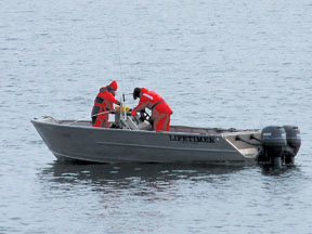
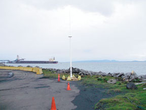
locations. The photos displayed were taken during this temporary deployment,
and show the SeaSonde antenna propped up sufficiently by a simple makeshift stand, and the boat loaded with transponder which was
used inside of the calibration and site quality analysis procedures.
Permanent installation of this network will occur once the electrical
power is brought to the sites later this summer.
For further information on SeaSondes in Canada, contact CODAR’s
local sales and technical services partner: Dr. Brian Whitehouse,
President, OEA Technologies Inc, Halifax, Canada,
E-mail: [email protected] |
 |
 |
Antenna Patterns Made Even Easier
|
 As the use of HF radar current maps for operational purposes such as search and rescue and spill
response is increasing, so too is the need to ensure that each system is producing the highest
quality data products possible. One of the most important steps operators can take to this
end is to measure the directional response of the receive antenna, referred to as its pattern.
While HF antennas leave the factory perfect, they will have interaction with the near-field
environment, altering its pattern. This interaction, which occurs with all HF antennas, has been
both understood and dealt with for decades. At CODAR, we have worked to streamline this
antenna pattern measurement (APM) process over the years to make it easier both to perform the
measurement and implement the field pattern data in real-time processing, as part of the calibration
process. With the only commercially available HF transponder and a suite of user-friendly software to process the signal, it
can take as little as an hour to begin processing data with a fully-calibrated SeaSonde antenna pattern. As the use of HF radar current maps for operational purposes such as search and rescue and spill
response is increasing, so too is the need to ensure that each system is producing the highest
quality data products possible. One of the most important steps operators can take to this
end is to measure the directional response of the receive antenna, referred to as its pattern.
While HF antennas leave the factory perfect, they will have interaction with the near-field
environment, altering its pattern. This interaction, which occurs with all HF antennas, has been
both understood and dealt with for decades. At CODAR, we have worked to streamline this
antenna pattern measurement (APM) process over the years to make it easier both to perform the
measurement and implement the field pattern data in real-time processing, as part of the calibration
process. With the only commercially available HF transponder and a suite of user-friendly software to process the signal, it
can take as little as an hour to begin processing data with a fully-calibrated SeaSonde antenna pattern.
Going back beyond 30 years, the traditional method for APM includes
mounting a transponder device to a small boat, airplane or helicopter which
makes a pass along an arc trajectory around the HF antennas. As streamlined
as this process has become, however, developing an automated method for
APM collection will be even simpler and increase the likelihood that a
system remains calibrated, in accordance with best practices guidelines.
|
.") In 2010, CODAR, in partnership with Brian Emery and Libe Washburn of
the University of California Santa Barbara, was awarded a Phase I SBIR from
NOAA to develop a method for automatically making antenna pattern
measurements by combining Automatic Identification System (AIS) data and
HF Doppler echoes of passing vessels. With the installation of a VHF
receiver collecting vessel speed, direction and position broadcast from its
AIS transponder, each vessel Doppler echo can be associated with its vessel’s
bearing. This is intended to run in real-time alongside standard surface
current processing. While transponder-based pattern measurements will still
be recommended during installation or in time-critical situations, an
automated process such as this under development will save time and money
on maintenance measurements and could even warn operators when a
pattern may have changed. The SBIR Phase I funding has provided the
opportunity to prove the feasibility of this method and now Phase II funding
is being sought to bring this technology to market. In 2010, CODAR, in partnership with Brian Emery and Libe Washburn of
the University of California Santa Barbara, was awarded a Phase I SBIR from
NOAA to develop a method for automatically making antenna pattern
measurements by combining Automatic Identification System (AIS) data and
HF Doppler echoes of passing vessels. With the installation of a VHF
receiver collecting vessel speed, direction and position broadcast from its
AIS transponder, each vessel Doppler echo can be associated with its vessel’s
bearing. This is intended to run in real-time alongside standard surface
current processing. While transponder-based pattern measurements will still
be recommended during installation or in time-critical situations, an
automated process such as this under development will save time and money
on maintenance measurements and could even warn operators when a
pattern may have changed. The SBIR Phase I funding has provided the
opportunity to prove the feasibility of this method and now Phase II funding
is being sought to bring this technology to market.
|
| Visit The Newly Improved CODAR Support Web Area
support.seasonde.com |
We are pleased to announce that our rapidly expanding collection of technical documents, photos and video tutorials has been
given a functional “facelift” that includes a web-based “Search Tool” for locating documents and tutorial videos quickly. The
CODAR knowledge base is divided into several general categories that are delineated by the disclosure bars shown in the illustration
below. The “Recent Additions” disclosure bar provides quick links to the most recent additions for savvy users who want to stay up-todate
with HF radar technology and SeaSonde products. The “SeaSonde Information” disclosure bar reveals sub-sections covering
SeaSonde principles of operation, site selection, site preparation and installation, while another reveals links to materials about
operational issues, data acquisition and QA/QC of data. SeaSonde owners will be also be pleased to know that our new site will have data
upload/download capabilities for transferring diagnostic and data file samples.
One of the most rapidly expanding
features is the number of video
tutorials. Our goal is to have short
5-10 minute video tutorials for the
most widely requested topics. Our
current focus for video production is
“How to’s” for setting up our new
Dome Transmit/Receive SeaSondes.
A link to the written dialog (in
English as a pdf file) is available to
assist our clients whose first language
is not English. In the future,
CODAR’s YouTube Channel will
mirror these antenna setup videos
making them available in the faststreaming
YouTube format. CODAR’s
official YouTube channel is: http://www.youtube.com/user/CodarOceanSensorsLtd.
All sections of the knowledge base
will remain open to the public except
for access to software releases,
administrative forms and private
client upload/download access.
|
 |
Register For SeaSonde Fall 2011 Training |
The next SeaSonde Training event takes place in Bodega Bay, California 10-13 October 2011. This course is
recommended for new SeaSonde operators and is a good refresher for experienced users as well. Event details
and registration form can be found at http://www.codar.com/CODAR_training_15_Fall_2011.shtml
|
How CODAR Deals with Interference
Every radar must detect target echoes against a background of unwanted noise. In our case, desired echoes may be first-order
Bragg scatter (from which we get current and tsunami information); second-order (from which sea state is obtained); or ship
echoes. Normal background in microwave radars is “white” Gaussian noise. White means that -- in the absence of echoes -- it is
flat in frequency space. Much of the time at HF we see and deal effectively with Gaussian noise. However, all too often we see
much more. Because HF radar is our only business at CODAR, we stay on top of it. Our science team has developed special,
effective methods to deal with this additional unwanted background, which we refer to as interference.
We review all four of
them here:
Ship-Type Echo Removal: Ship velocities span the same Doppler region as sea echoes. When present, they interfere with
accurate sea-surface information extraction. Over 25 years ago, we developed an algorithm to detect and get rid of ship-type
echoes. It is based on the fact that a ship with given radial velocity stays in a given Doppler bin only for a predictable period of
time, based on the size of the range cell and the radar frequency. If a “blip” suddenly appears in Doppler spectral bins of interest,
we test for these properties: does it stay in the bins for the correct time, or for much longer? If the former, then those bins get
withheld. If much longer, then we conclude that the background has risen to a new level, and we must live with it, not withhold it
or the data will get unacceptably stale. In that case, normal white Gaussian noise thresholding methods are applied. This
algorithm has been used successfully well over two decades, yielding good current and wave data that are not contaminated by
outliers due to these frequent “ships passing in the night” (or similar types of longer-duration interferers).
Time scale for ship-type echo interference: Several minutes.
Ionospheric-Type Echo Rejection: When our lower-frequency radars began seeing beyond 90 km about 12 years ago, we faced
another nuisance. Echoes from the ionosphere directly overhead spanning from 90 km - 300 km might be seen at certain times
of the day and night. These layers of charged particles ionized by the daytime sun act like a mirror. Often (but not always) they
are restricted to two or three range cells, but they can be spread over many Doppler bins because the ionosphere is in motion.
We developed an algorithm to find and excise this type of interference. It has been optimized by over a decade of experience.
The algorithm knows what to look for, and simply removes all data from the offending range cell and Doppler bins. Often this is
necessary only on one side of the positive/negative Doppler span (which fortunately contain redundant current and wave
information), so that a range gap does not always occur. Without this algorithm, obviously wild “current” vectors would have
appeared, spread in angle across the entire range cell -- an unacceptable contamination.
Time scale ionospheric-type echo interference: Half hour to two hours.
Impulse Removal: Much external noise seen at HF comes from the atmosphere: thunderstorms worldwide generate radio noise
that originate far away. Typically 2000 thunderstorms are active in the world at any given time, producing 100 lightning strikes
per second. When these lightning sources are distant, they add up to a noise that looks continuous and Gaussian. Those closer to
the radar are impulsive in nature, and Gaussian methodologies no longer work in this case. A single blast from a nearby strike can
ruin an entire Doppler spectrum collected over several minutes, even though the impulse duration is only a millisecond. Some
time ago CODAR developed and optimized an impulse detector, done after range processing before Doppler processing (typically
every 0.5 - 1 second). When it detects a burst exceeding a preset threshold above the background, it excises that time sample and
replaces it with an interpolated value across this gap. An example of “before and after” is shown below for West Florida, which is
“thunderstorm alley” among our U.S.-based SeaSondes and was used in this development. This technique can reduce impulsive
background interference as much as 15-20 dB when storms are nearby.
Time scale for impulse noise interference: Less than a second.
Plot of signal strength (color) vs. time
(horizontal axis) and range (vertical
axis) showing four lightning/impulsive
interference bursts over 256 seconds. |
 vs. time (horizontal axis) and range (vertical axis) showing four lightning/impulsive interference bursts over 256 seconds.") |
 |
Sea-echo Doppler spectrum
contaminated by the impulse bursts
shown in prior time series. |
 |
Acceptable sea-echo Doppler
spectrum after excision of impulses in
first time-series panel. |
• Radio Station Interference Rejection: The HF band has been used historically for radio communication and broadcasting
-- HF radar is a newcomer to the this frequency region. Although radio broadcasters as well as radars have frequency licenses, all
too often distant radio stations interfere with us. These may be radiating illegally, or may result from unavoidable duplication of
authorizations on the same channel because of the scarcity of separate spectral spaces for everyone. Usually the signals that
interfere with us are propagated by skywave (purposely reflecting from the ionosphere), because this is where HF excels for radio
broadcasters by reaching great distances. They therefore adjust their frequency throughout the day to take advantage of the best
propagation conditions. As a result, when we hear radio interference, it typically may last for a couple hours before the
broadcaster moves on to a more favorable frequency. With the FMCW modulation that we all use, these interfering radio signals
appear spread in range but confined in Doppler. Therefore, they can at times look like a Bragg peak, second order echoes, or
mask a ship while appearing like a ship echo themselves. However, based on their range-spread nature, we can identify and deal
with them. This is done by recognizing that -- because of our I/Q processing -- radar echoes are seen only for “positive” range
cells, while interference bands appear symmetrically at both positive and negative ranges. Unlike others, we don’t simply subtract
all negative from positive cells, for this too often actually increases other types of background interference. We do a careful search for the expected patterns of this radio-signal interference, subtracting just that portion, but only if it exceeds a threshold
based on background levels and expected I/Q balances. Check out the example below to observe how effective this can be, when
done properly.
Time scale for radio signal interference: A broadcaster may use a given frequency for two-three hours. The interfering constantrange
bands will move in Doppler spectral position every processing period (e.g., 4 - 17 minutes).
Color spectral plot on left shows
significant vertical interference stripes
over range, with radial velocity from
the Doppler spectral shift as the
horizontal axis, for the three antennas
of the 13 MHz SeaSonde at Nordoy in
Norway. Plot on right shows same
spectra using suppression method
described here. The first and second
order Bragg areas are seen more
clearly, and several ship echoes are
uncovered when this interference is
excised. The very top of the right
plots purposely retains nterference
levels before removal for reference. |
 |
|


|
 |
| |
1914 Plymouth Street
Mountain View, CA 94043 USA
Phone: +1 (408) 773-8240
Fax: +1 (408) 773-0514
www.codar.com |
 |
|
|

 to the West, the Sea of Japan (East Sea) to the East and the East China Sea and Korea Strait to the SouthSouth Korea is nearly surrounded by water with the Yellow Sea (West Sea) to the West, the Sea of Japan (East Sea) to the East and the East China Sea and Korea Strait to the South")
